
BigQuery allows you to query large amounts of data in a very short amount of time. Being a Google-managed service, the user doesn’t have to worry about configuring the database and/or architecture. Nevertheless, the user must pay attention to how the data is saved and how to write the queries in order to get the best performance from BigQuery. In fact, it must be remembered that the service is paid and the cost depends on the resources required.
In this article we will analyze best practices to reduce costs and improve BigQuery response times.
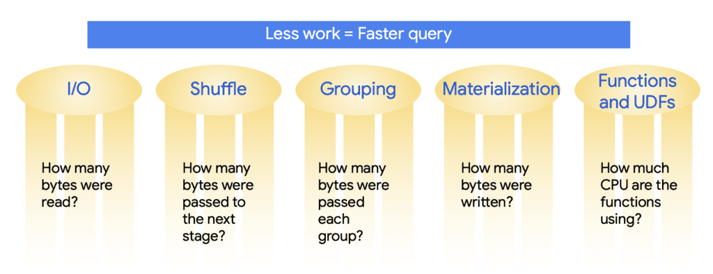
There are five key areas for performance optimization in BigQuery and they are:
- Input/output: how many bytes have been read from the disk
- Shuffling: how many bytes have been passed to the next stage of query processing
- Grouping: how many bytes were passed to each group
- Materialization: how many bytes have been permanently written to disk
- Functions and UDFs: how computationally expensive the query is in CPU terms
How to write queries
Based on the five areas previously introduced, let’s look at “tricks” to apply when writing queries.
To reduce the number of data reads, don’t select more columns than necessary. This means avoiding SELECT * as often as you can. Also, insert filters in the WHERE clause as early and often as possible. This will reduce the amount of data.
In case you have a really huge dataset, consider using approximate aggregation functions instead of regular ones. These, in fact, are much faster to execute and require less CPU. The downside is that the statistics will be approximate. In some cases, however, this can be accepted.
Limit the use of the ORDER BY clause to the outermost query, avoiding data sorting in the intermediate steps. For example, in temporary tables defined using the WITH clause, sorting should not be performed. You can find it in some examples only associated with aggregation windows as seen in article BigQuery: WINDOWS analytics.
Avoid JOINs as much as possible. If they are necessary, put the largest table on the left. This will help BigQuery optimize the operation. If you forget, BigQuery will probably do these optimizations for you, so you may not even see any difference.
You can use wildcards in table suffixes to query multiple tables, but try to be as specific as possible with these wildcards.
The attributes to be included in the GROUP BY clause are the ones that should be displayed without aggregation functions in the SELECT. Be careful, however, to choose attributes with few distinct values.
Finally, it is possible to partition the tables, as we will see in the next section.
Below is the cheat sheet of best practices.

Table partitioning
One of the ways you can optimize the tables in your data warehouse is to reduce the cost and amount of data reads by partitioning your tables.
For example, suppose you partitioned the table shown in the figure below using the eventDate column. BigQuery will organize its internal storage so that dates are stored in separate shards. Each partition, for example, will contain data for a single day. When data is stored, BigQuery ensures that all data within a block belongs to a single partition. A partition table maintains these properties for all operations that modify it: queries, DML statements, DDL statements, load and copy data tasks. This requires BigQuery to maintain more metadata than an unpartitioned table.
As the number of partitions increases, the amount of metadata increases. The benefit, however, results in the reduction of resources required for certain queries. For example, if a query includes only the dates between January 3 and January 4 in the WHERE clause, BigQuery will only need to read two-fifths of the entire dataset. This can result in drastic savings in cost and execution time.

There are two main ways to partition tables in BigQuery. When inserting data into the target table for the first time or using a column that is already there. The figure below shows the commands to perform partitioning.

The first example shows how you can create a table that uses day-based partitioning at the time of data ingest. BigQuery automatically creates new date-based partitions without any additional maintenance. In addition, you can specify the expiration time for the data in the partitions.
The other two cases, however, use an existing column on an already defined table as the partitioning key. The columns must be of type date, timestamp or a column on which integer numeric ranges can be defined. In the example shown, you are partitioning based on the customer_id field by defining a range of values between 0 and 100 in increments of 10.
Although you need to maintain more metadata by making sure the data is partitioned globally, BigQuery can more accurately estimate the processed bytes of a query before executing it. This cost calculation provides an upper bound on the final cost of the query. A good practice is to write queries always including the partition-related filter. You must make sure that the partition field is isolated on the left side, as this is the only way BigQuery can quickly discard unnecessary partitions. Below is an example of how to include the partition reference.

Clustering
In addition to partitioning, you can also use clustering. Currently, BigQuery only supports clustering on partitioned tables. This type of data clustering can improve performance for certain types of queries, such as queries that use filter clauses and those that aggregate data on the attribute used to define the cluster. Once the data is written to a cluster table, BigQuery sorts the data using the values in the clustering columns. These values are used to organize the data, some multiple blocks, and BigQuery’s storage.
When submitting a query containing a filter on the data in the clustering columns, BigQuery uses assorted blocks to eliminate unnecessary data scans. Similarly, when a query aggregates data based on clustering column values, performance is improved because the sorted blocks locate rows with similar values.
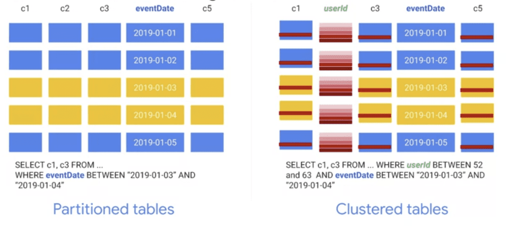
In the example shown in the figure, the tables are partitioned by eventDate and clustered by userId. Since the query filters the data based on a specific eventDate range, only two of the five partitions are considered. In addition, the query searches for users who have an identifier in a specific range. Therefore, BigQuery can jump to the selected row range and read only those rows for each of the columns requested in the query.
Clustering is set when the table is created. The creation of the table used in the previous example is defined with the following command.
CREATE TABLE mydaset.mytable(
    c1 NUMERIC,
    userId STRING,
    eventDate TIMESTAMP,
    c5 GEOGRAPHY
)
PARTION BY DATE(eventDate)
CLUSTER BY userId
OPTIONS (
    partition_expiration_days=3,
    description='cluster')
AS SELECT * FROM mydaset.othertable;
In addition to the definition of partitioning and clustering, the statement specifies for BigQuery to expire partitions that are more than three days old.
The columns used for clustering locate related data. When clustering a table using multiple columns, the order of the columns is important because it determines the ordering of the data itself. In theory, as changes are made to the table, the degree of data sorting begins to weaken, which causes the data to be partially sorted. Therefore, if the table is partially sorted, queries using clustering columns may need to scan more blocks than when the table is fully sorted.
You can re-cluster the data in the entire table by running a query that selects everything and re-writes it in the table itself. This operation, however, is no longer necessary!!! In fact, BigQuery now periodically does automatic re-clustering for free.


