In the previous articles, BigQuery: WITH clause and BigQuery: GIS functions and Geo Vis, we looked at some of BigQuery‘s functionality. Specifically, we looked at the WITH construct to improve query readability and split the problem into subqueries. Furthermore, through GIS functions we saw how to use geographic data both to calculate some metrics and to visualize them with Geo Vis. The queries we wrote, however, did not require complex analysis.
In many cases, however, the analysis to be performed requires partitioning the initial data set into subsets and, for each of these, calculating appropriate statistics. To perform this type of operation, it is necessary to use analytical windows.
To better understand their syntax and operation, in this article we will analyze the dataset of the bike sharing in the city of London to extract some information that may be useful for the manager of the service.
Dataset
The dataset that will be used in the following scenarios is for the City of London’s bike sharing service. As already described in article BigQuery: GIS functions and Geo Vis, it consists of two tables, one relating to all trips made by the bikes in the fleet, the other containing station-specific information (including geographic information).
The number of trips recorded within the dataset is about 24 million, covering the trips of about 100 stations.
Scenario 1: station utilization
The first analysis we want to perform relates to the average time that bikes remain idle at each station before being picked up by another rider. This could help, for example, the service manager avoid running out of inventory for high demand stations. Or, the marketing team could set up a program to incentivize bike rentals from slower turnover stations versus high demand stations. The uses can be truly multifaceted.
As in the example in article BigQuery: GIS functions and Geo Vis, we will use a staging table to merge station information with trip information. At this point, however, we need to find a way to “look back” and observe the previous time a bike (identified by the bike_id field) was returned to that station. Having found the method, we will simply need to run the difference between the timestamps to get the idle time.
To look back in time, we can use the LAG function. This function returns, by default, the value of the field passed as the previous line parameter. You can also pass an offset parameter to define the previous row number to return. In this case we will pass the end_date field of the bike structure. For the delay to make sense for our analysis, however, we must use an analytic function to logically split the data before performing the calculation.
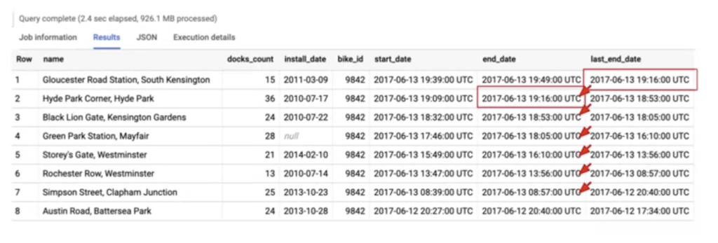
The LAG function will need to be applied to different subsets of data. To make sure that the function is not applied to the result of the WHERE and GROUP BY clauses, but to a variant of it, we need to specify the OVER clause. Within it, to partition the data properly, we use the PARTITION BY clause. In this case we partition the data by bike_id and sort the data within each partition by start_date from oldest to newest. This allows us to traverse past rentals accurately. In the figure you can see a partition and how the LAG function calculates the result.

Finally, we apply the TIMESTAMP_DIFF function between the current start time of the rental and the end time of the last rental to obtain the time in hours that the bike was idle at that station. We can then aggregate for each station name and calculate the average idle time. For completeness, we also calculate the number of rentals and include the number of available spots for each station and the date the station was installed. Obviously, to display this station information as well, we need to include the related attributes in the GROUP BY clause as well.
For better readability, we can sort the data by unused time and show the first 10 results.
The resulting query is as follows.
WITH staging AS (
  SELECT
    STRUCT(
      start_stn.name,
      ST_GEOGPOINT(start_stn.longitude, start_stn.latitude) AS point,
      start_stn.docks_count,
      start_stn.install_date
    ) AS starting,
    STRUCT(
      end_stn.name,
      ST_GEOGPOINT(end_stn.longitude, end_stn.latitude) AS point,
      end_stn.docks_count,
      end_stn.install_date
    ) AS ending,
    STRUCT(
      rental_id,
      bike_id,
      duration, -- seconds
      ST_DISTANCE(
        ST_GEOGPOINT(start_stn.longitude, start_stn.latitude),
        ST_GEOGPOINT(end_stn.longitude, end_stn.latitude)
        ) AS distance, -- meters
      ST_MAKELINE(
        ST_GEOGPOINT(start_stn.longitude, start_stn.latitude),
        ST_GEOGPOINT(end_stn.longitude, end_stn.latitude)
        ) AS trip_line, -- straight line (for GeoViz)
      start_date,
      end_date
    ) AS bike
  FROM `bigquery-public-data.london_bicycles.cycle_stations` AS start_stn
  LEFT JOIN `bigquery-public-data.london_bicycles.cycle_hire` AS b
  ON start_stn.id = b.start_station_id
  LEFT JOIN `bigquery-public-data.london_bicycles.cycle_stations` AS end_stn
  ON end_stn.id = b.end_station_id
),
lag_end_date AS (
-- Find how long after one ride ends, another one begins (on average)
SELECT
  starting.name,
  starting.docks_count,
  starting.install_date,
  bike.bike_id,
  LAG(bike.end_date) OVER (
    PARTITION BY bike.bike_id
    ORDER BY bike.start_date)
  AS last_end_date,
  bike.start_date,
  bike.end_date
FROM staging
)

SELECT
  name,
  docks_count,
  install_date,
  COUNT(bike_id) AS total_trips,
  ROUND(
    AVG(
      TIMESTAMP_DIFF(start_date, last_end_date, HOUR)
      )
  ,2) AS time_at_station_hrs
FROM lag_end_date
GROUP BY
  name,
  docks_count,
  install_date
HAVING total_trips > 0
ORDER BY time_at_station_hrs ASC -- fastest turnover first
LIMIT 10;
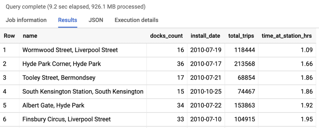
The result we get is shown below.

Scenario 2: bike maintenance
The bike sharing operator must also keep its fleet in good condition. If a bike is broken, it will no longer be used and therefore represent a loss for the operator.
We can base our analysis on the usage of each bike. Those most used will have a higher probability of needing to be fixed and/or checked. Starting with the staging query to merge trip information with station information, we assign a score to each trip of each bicycle. We give a score of one to the first trip made, two for the second trip, and so on. To do this, we use the RANK function. This must be applied to each partition defined by the bike identifier (bike_id). In order for the score to be correct, we need to sort the data within each partition by the start date of the trip (bike.start_date).
In addition to this score, we also calculate the cumulative distance and duration for each bike. We then use the same partition and sorting for the two new measures. The duration, expressed in hours, will be calculated using the SUM(bike.duration/60/60) function, while the distance, expressed in km, will be calculated using the SUM(bike.distance/1000) aggregation function. We group all this information in a stats structure using the STRUCT clause.
The result is what was required of us. However, it is quite time consuming to examine the 24 million records to identify the bikes that need maintenance. So we need a general ranking of the bicycles based on their statistics without losing the details calculated so far. How can we proceed? The solution is to use the ARRAY data type.
We group the result of the previous query according to the identifier of the bikes and assign a score (RANK function) based on the distance covered. To get this information, since we only have the cumulative values, we need to use the MAX function. The rank will then be applied on the data sorted according to the values returned by the function MAX(stats.cumulative_distance_km). This type of window defines a logical partition and not a column partition as seen above.
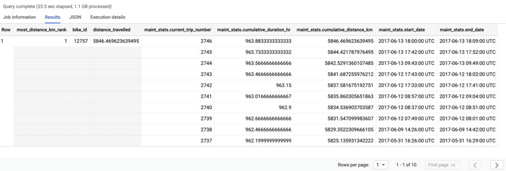
To define an array, simply use the ARRAY_AGG clause. In this case, we associate with each bike the detailed statistics of each trip that we calculated earlier. We can also sort the data inside the array by the date the trip ended and limit the number of elements inside the array. Arrays are extremely useful in BigQuery because they allow us to define multiple levels of granularity on the data.
WITH staging AS (
  SELECT
    STRUCT(
      start_stn.name,
      ST_GEOGPOINT(start_stn.longitude, start_stn.latitude) AS point,
      start_stn.docks_count,
      start_stn.install_date
    ) AS starting,
    STRUCT(
      end_stn.name,
      ST_GEOGPOINT(end_stn.longitude, end_stn.latitude) AS point,
      end_stn.docks_count,
      end_stn.install_date
    ) AS ending,
    STRUCT(
      rental_id,
      bike_id,
      duration, -- seconds
      ST_DISTANCE(
        ST_GEOGPOINT(start_stn.longitude, start_stn.latitude),
        ST_GEOGPOINT(end_stn.longitude, end_stn.latitude)
        ) AS distance, -- meters
      ST_MAKELINE(
        ST_GEOGPOINT(start_stn.longitude, start_stn.latitude),
        ST_GEOGPOINT(end_stn.longitude, end_stn.latitude)
        ) AS trip_line, -- straight line (for GeoViz)
      start_date,
      end_date
    ) AS bike
  FROM `bigquery-public-data.london_bicycles.cycle_stations` AS start_stn
  LEFT JOIN `bigquery-public-data.london_bicycles.cycle_hire` AS b
  ON start_stn.id = b.start_station_id
  LEFT JOIN `bigquery-public-data.london_bicycles.cycle_stations` AS end_stn
  ON end_stn.id = b.end_station_id
)
-- Collect key stats for each bike on total usage
, maintenance_stats AS (
SELECT
  bike.bike_id,

STRUCT(
  RANK() OVER(
    PARTITION BY bike.bike_id
    ORDER BY bike.start_date
    ) AS current_trip_number,

  SUM(bike.duration/60/60) OVER(
    PARTITION BY bike.bike_id
    ORDER BY bike.start_date
    ) AS cumulative_duration_hr,

  SUM(bike.distance/1000) OVER(
    PARTITION BY bike.bike_id
    ORDER BY bike.start_date
    ) AS cumulative_distance_km,

  bike.start_date,
  bike.end_date
  ) AS stats
FROM staging
)
SELECT
  -- High level summary
  RANK() OVER(
    ORDER BY MAX(stats.cumulative_distance_km) DESC
    ) AS most_distance_km_rank,
  bike_id,
  MAX(stats.cumulative_distance_km) AS distance_travelled,
  -- Detail within array (show 10 most recent rides)
  ARRAY_AGG(stats ORDER BY stats.end_date DESC LIMIT 10) AS maint_stats
FROM maintenance_stats
GROUP BY bike_id
ORDER BY most_distance_km_rank
LIMIT 10;
While the result we get is as shown below. Beware that although it looks like several rows, it is technically just one record. In fact, the cells on the left are grayed out, which means that the initial values are valid for all the tuples in the array.


