Unlike relational databases, MongoDB allows you to create pipelines for manipulation and extraction of statistics in a simple and intuitive way. With the latest versions, the aggregation pipeline was introduced, which is based on the idea of creating a data processing framework. Documents in a collection enter a multi-step pipeline that transforms the documents into an aggregated result. Operations in each step allow, for example, values from multiple documents to be grouped together, statistics to be calculated, and information from other documents to be integrated with the goal of returning a single result.
In this tutorial we are going to explore some of the most used and useful operations proposed by the aggregation framework through examples. We will take advantage of the example databases provided with the free installation of MongoDB Atlas and build pipelines using the graphical interface provided by MongoDB Compass. To get completely free cloud environment to practice you can refer to the article MongoDB Atlas – creating a cloud environment for practice. On the other hand, if you already have your MongoDB Atlas available, you can refer to article MongoDB Compass – easily query and analyze a NoSQL database to find out how to connect to the cloud, practice some queries and practice using the MongoDb Compass tool.
Extracting statistics
The aggregation pipeline is very often used to extract statistics. For this example we will use the sample_training database and in particular the grades collection. Each document of this collection contains the id of the student, the id of the class and a vector of embedded documents consisting of a type field and a score.
If you wanted to find the average score for each score type, you would need to use an aggregation pipeline. MongoDB Compass allows us to create the aggregation pipeline interactively, verifying that the result of each stage is correct both syntactically and at the level of the set of documents returned. To start familiarizing yourself with this data extraction methodology or to test complex queries this is the best tool.

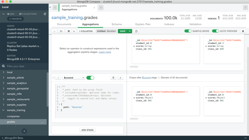
Returning to the example, first we need to unpack the scores vector so that our calculation is performed on all the scores included in each document. For this reason we use the $unwind operator. As you can see from the figure, on the left we will define the operator and the parameters that are required, while on the right, as soon as the pipeline block is properly configured, we will get a preview of the documents returned by the stage in question (the AUTO PREVIEW option must be active). The stage will be defined as follows:
{path: "$scores" } Attention
The $ symbol before the attribute name is used to indicate that you want to use the values inside the field. For the $unwind operator this symbol must always be present.
What you get is a document for each element of the scores vector. Each document will have the same fields of the original document but the score field will be an embedded document related to the i-th element extracted.
At this point we can calculate the statistics of interest by defining groups of interest and specifying the measures to be calculated. The operator to perform this operation is $group. We then add a stage by clicking on the ADD STAGE button or on the + button at the top right of the current stage. As before, we will select the $group operator and define its respective parameters. In the example case it is necessary to group by score_types. Therefore the _id of the document exiting the $group stage will be equal to the value of the score_type field. To calculate the average we’ll define a new field that will be calculated with the $avg operator with respect to the values contained in the scores.score path. The stage will look like this
{
  _id: "$scores.type",
  avg: {$avg: "$scores.score"}
}
Obviously other statistics can be extracted such as the minimum, maximum and number of items in each group.
{
  _id: "$scores.type",
  avg: {$avg: "$scores.score"},
  min: {$min: "$scores.score"},
  max: {$max: "$scores.score"},
  count: {$sum: 1}
}
Attention
For counting the number of items in each group, the $sum operator must be used to increment a counter by 1 each time a document is associated with a group. This is because the $count operator is used to define a stage that counts the number of incoming documents received.
It is possible to export the pipeline defined in some programming languages (Python, Java, Node, C#) or simply copy it and then use it in the shell by clicking on the button ![]() . The final result will be as follows:
. The final result will be as follows:
[{$unwind: {
  path: '$scores'
}}, {$group: {
  _id: '$scores.type',
  avg: {
    $avg: '$scores.score'
  },
  min: {
    $min: '$scores.score'
  },
  max: {
    $max: '$scores.score'
  },
  count: {
    $sum: 1
  }
}}]
Quantile analysis
The aggregation pipeline structure of the previous example can be used whenever it is necessary to extract some standard statistics about the distribution of the data. Sometimes, however, it is necessary to compute quantiles.
In statistics and probability, quantiles are cut points dividing the range of a probability distribution into continuous intervals with equal probabilities, or dividing the observations in a sample in the same way. q-quantiles are values that partition a finite set of values into q subsets of (nearly) equal sizes. There are q − 1 of the q-quantiles, one for each integer k satisfying 0 < k < q.
Wikipedia
There are some quantiles, defined as simple order, that are very common in statistics. These include:
- median: order 1/2
- quartiles: orders 1/4, 2/4 and 3/4
- deciles: of order m/10
- centiles (or percentiles): order m/100.
Calculating these measures requires ordering the data of interest and then calculating exactly the order of the corresponding quantile.
For this example we will use the sample_airbnb database and focus on calculating some price-related quantiles. Specifically, we will calculate the median, the first and fourth quartiles, and the 95th percentile.
The first step is to sort the data in the collection.We will use the $sort operator. Similarly to the sort function used to sort the results of the find, the $sort operator requires a sorted document of the attributes on which to perform the sort. For each of them it is mandatory to insert the direction of the sort (1 ascending, -1 descending). In our example we will have to order the price field in ascending order as shown below.
{$sort: {
  price: 1
}}
To proceed with the calculation of quantiles, we need to group all the values of the price field into a vector. In this way we can exploit the calculation operators on vectors to extract the values of the quantiles of interest.
We then need to group all the documents in the collection into a single document that will contain a value vector containing all the sorted price values. The _id of the $group operator will be set to null to obtain a single document representing the entire collection, while the $push operator will insert the value of the price field for each document resulting from the previous step. The sorting by price will be preserved as the documents will be read sequentially. The $group stage will be defined as follows.
{$group: {
  '_id': null,
  'value': {'$push': '$price'}
}}
The calculation of quantiles will be done by some mathematical and vector manipulation operators. In particular, we will use the operators
Using the $size operator we will calculate the size of the value vector. Obviously it was possible to extract this information during the grouping operation using the $sum operator. The size of the vector will have to be multiplied by the value of the quantile of interest. For example, if we want to calculate the median we will have to multiply it by 0.5, for the first quartile by 0.25, and so on.
The result of this multiplication will be the position within the vector where we will find the value of the quantile. Since the position must be an integer, we need to ensure that the returned value does not contain any decimals using the $floor operator. This operator takes the largest integer less than or equal to the specified number. This can then be extracted to the calculated position of the array corresponding to the quantile using the $arrayElemAt operator.
These calculations will need to be repeated for each quantile to be calculated and placed within a $project stage. This last stage will look as follows.
{$project: {
  _id: 0,
  "0.25": {
    $arrayElemAt:
    ["$value",
    {$floor: {$multiply: [ 0.25, {$size: "$value"} ] } }
    ]
  },
  "median": {
    $arrayElemAt:
    ["$value",
    {$floor: {$multiply: [0.5, {$size: "$value"} ] } }
    ]
  },
  "0.75": {
    $arrayElemAt:
    ["$value",
    {$floor: {$multiply: [0.75, {$size: "$value"} ] } }
    ]
  },
  "95": {
    $arrayElemAt:
    ["$value",
    {$floor: {$multiply: [0.95, {$size: "$value"} ] } }
    ]
  }
}
Time analysis
MongoDB can be used to store time series data. For maximum performance, it is necessary to define document patterns that minimize disk occupancy and optimize access of time series related to the same measurement object. A more in-depth discussion on how to appropriately model documents can be found here.
The fields of application are therefore many. They range from sensor measurements in the Internet of Things (IOT) field to event tracking of an information system. In the sample databases provided in MongoDB Atlas we find the sample_weatherdata database. Although the document structure does not reflect time series modeling directions, it is a great example to practice with the aggregation framework to extract statistics relative to time.
Suppose we need to extract for each time interval the minimum and maximum temperatures if there were more than 10 detections. In this case we will initially need to group by the ts field and calculate the measurements of interest. The first stage of the aggregation pipeline will then result:
{$group: {
  _id: "$ts",
  minTemp: { $min: "$airTemperature.value"},
  maxTemp: { $max: "$airTemperature.value"}
  }
}
The result of this stage will be a set of documents where each represents an instant in time with its associated temperature measurements. However, the number of measurements, i.e., documents, that belong to each group is not considered. In order to exclude documents that do not meet the required condition we need to insert an additional measure in the $group stage: the number of items belonging to each group. To do this, just enter the count measure as seen in the previous example.
{$group: {
  _id: "$ts",
  minTemp: { $min: "$airTemperature.value"},
  maxTemp: { $max: "$airTemperature.value"},
  count: {$sum: 1}
  }
}
Filtering based on the number of documents belonging to each group will be done using the $match operator.
{$match: {
    c: {$gt:10}
}}
The structure of this pipeline is very similar to what you do in SQL queries when you make a GROUP BY and then you insert the HAVING operator to filter the result. Unlike the SQL language where you can use aggregation functions (min, max, avg, count, sum) in the having and select clauses, in MongoDB you must define in the $group stage all the measures that will be used in subsequent stages. We must remember that the output of each stage of an aggregation pipeline is a set of documents that will play the role of input for the next stages.
In the example just discussed, the value of a specific field was used directly to define the time intervals. This is due to the fact of the data distribution of the analyzed collection. In many cases, however, it is required to define intervals derived from the timestamp saved in the documents such as the day of the week, the month or even the year. MongoDB offers the ability to easily extract this information from timestamps and insert it into the aggregation pipeline. We could almost compare this property to the Extract, Transform, Load (ETL) processes typical of data warehouses. Here is an example based on the sales collection of the sample_supplies database.
Suppose we want to calculate the total collection and the number of items sold for each month. The collection contains in the saleDate field only the timestamp relative to the time of purchase. It is therefore necessary to extract from this field the necessary information to define the intervals appropriately.
Attention
Time operators can only be applied on fields of type Date, Timestamp, and ObjectID. Also, each operator extracts only the information for which it was defined. For example, the $month operator will extract the numeric value of the month, while $year will extract the year. So if you want to group for each month you have to use both month and year. Otherwise months belonging to different years will not be distinguished.
To use the month and year information in the analyses we are going to perform, we need to add it to each document in the collection. However, it is not necessary to perform an update operation! We can use the $addFields stage to insert new attributes to each document and make this change available only within the aggregation pipeline. In this way we won’t increase the size of our database with information that can be computed effectively when needed, nor will we have to modify the applications that use the database to properly handle the new data structure. The first stage therefore will look as follows:
{$addFields: {
  month: { $month: "$saleDate" },
  year: {$year: "$saleDate"}
}}
The documents coming out of this stage will have a similar structure to the one below.

Since the request is to calculate some sales statistics, we need to decompose the items vector. This operation will be performed using the $unwind operator.
{$unwind: {
  path: "$items",
}}
Each document will then represent the sale of a single item. The information that was added at the beginning is retained. We can then group all documents belonging to the time interval of interest.
Since we haven’t defined a unique field that encompasses both month and year, we need to enter as the _id of the $group operator a document consisting of both fields. This operation is lawful and must be performed whenever the groups of interest are determined by combining the values of different attributes.
{$group: {
  _id: {month: "$month", year: "$year"},
  c: {$sum:1},
 income: {$sum: "$items.price"}
}
The resulting documents will have the following structure.


