In the field of machine learning there are several algorithms for clustering data. In the article DBSCAN: how it works, we analyzed DBSCAN, which provides very robust results when outliers and nonglobular shapes are present. Nevertheless, in some application contexts it cannot always be applied and/or its results are not optimal. In this paper we will explain another algorithm: the K-Means. It is a very popular clustering algorithm. Without going into the more technical and mathematical details of the approach, we will explain the intuition behind it.
Before we start with the algorithm, let’s review what clustering is. Clustering is the automatic discovery of natural groupings in data. Usually, when we are given data that we can visualize (2-dimensional or perhaps even 3-dimensional data), the human eye can easily form distinct clusters. But for PCs, it is a bit more difficult to do so. This is where clustering algorithms come in. They are also very useful when we have to handle data with a number of dimensions greater than 3 that even the human eye cannot visualize and cluster.
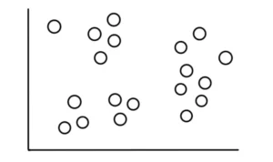
Imagine, then, that we have 19 points that look like this:
Now suppose we know that these data fall into 3, relatively obvious, categories that look like this:
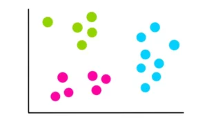
Our task is to use the K-means algorithm to perform this categorization.
Step 1: Select the number of clusters k
The number of clusters we want to identify is the k parameter of the algorithm. In this case, since we assumed that there are 3 clusters, k = 3.
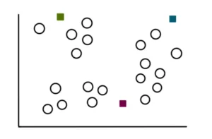
Step 2: Select k random points
The process of finding clusters begins with the selection of 3 random points (not necessarily our data points). These points will serve as centroids of the clusters we are going to create:
Step 3: Create k clusters
To create the clusters, we start by measuring the distance of each point from each of the 3 centroids. Then we assign the points to the closest cluster. Therefore, for a sample point, the distances will appear as follows:
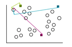
If we look closely, we see that the distance between the point and the green centroid is the least. Consequently, we assign the point to the green cluster.
In two dimensions, the formula for finding the distance between two points that is usually used is the Euclidean formula that is given below:
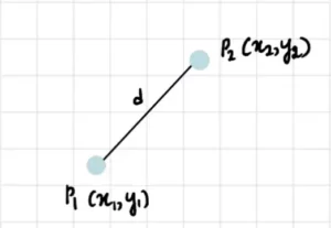
Of course, in some contexts other distance measures can be used, such as Manhattan’s, Minkowski’s, cosine or others. To best understand the algorithm we will use the Euclidean one.
Therefore, using the Euclidean measure discussed above, we repeat this process for the rest of the points. At the end of the process the clusters will look something like this:
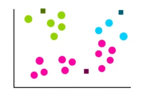
Step 4: Calculation of the new centroid of each cluster
Now that we have obtained our 3 clusters, we find the new centroids formed by each of them. For example, the way we calculate the coordinates of the centroid of the blue cluster is:
Where x1, x2 and x3 are the x coordinates of each of the 3 points in the blue cluster. And y1, y2 and y3 are the y coordinates of each of the 3 points in the blue cluster. We divide the sum of the coordinates by 3 because there are 3 data points in the blue cluster. Similarly, the coordinates of the centroids of the pink and green clusters are:
Thus, the new centroids will be:
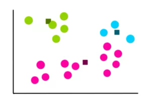
Step 5: Evaluate the quality of each cluster
Since k-means cannot see clustering as we do, it is necessary to measure the quality of the result obtained by finding the variation within all clusters. The basic idea of k-means is to define clusters so that the within-cluster variance is minimized. To quantify this variance, we calculate something called the sum of squares within cluster (WCSS):
where C are the centroids and d are the points in each cluster.
To simplify, we visually represent the variation in this way:
Step 6: Repeat steps 3-5
Once the previous clusters and variation are stored, we start over. But this time we use the previously computed centroids to create 3 new clusters, recompute the center of the new clusters, and compute the sum of the variation within all clusters.
Suppose the next 4 iterations look like this:
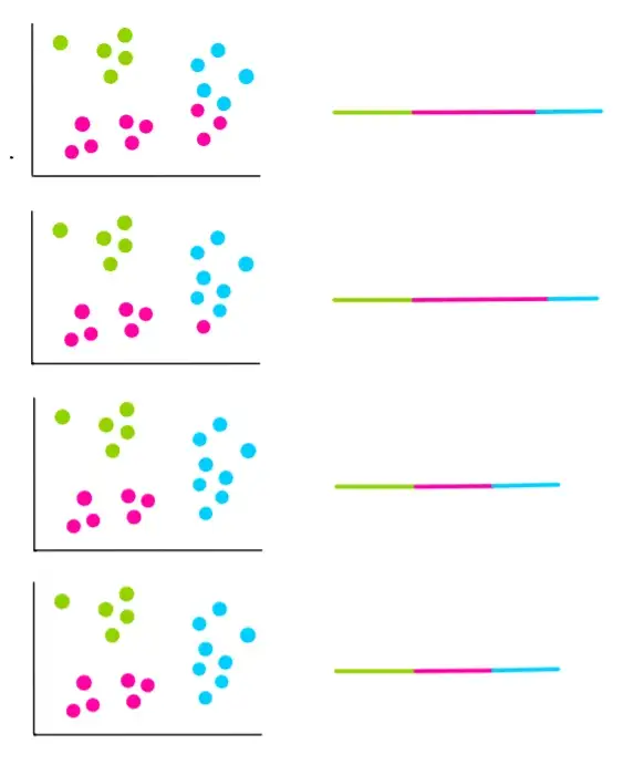
In the last two iterations, we can see that the clusters have not changed. This means that the algorithm is convergent and the clustering process is stopped. We then choose the clusters with the lowest WCSS, which in our example are those in the last two iterations.
How to choose k?
In our example, we knew that we needed 3 clusters. But if we don’t know how many clusters we have, how do we choose k?
In this case, we try different values of k and calculate the WCSS.
k=1

k=3

k=2

k=4
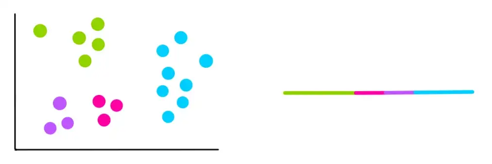
It can be seen that each time a new cluster is added, the total variation within each cluster is less than the previous one. And when there is only one point per cluster, the variation is 0. So to find the best k, we have to use an “elbow” graph, which relates the WCSS to the number of clusters or k.
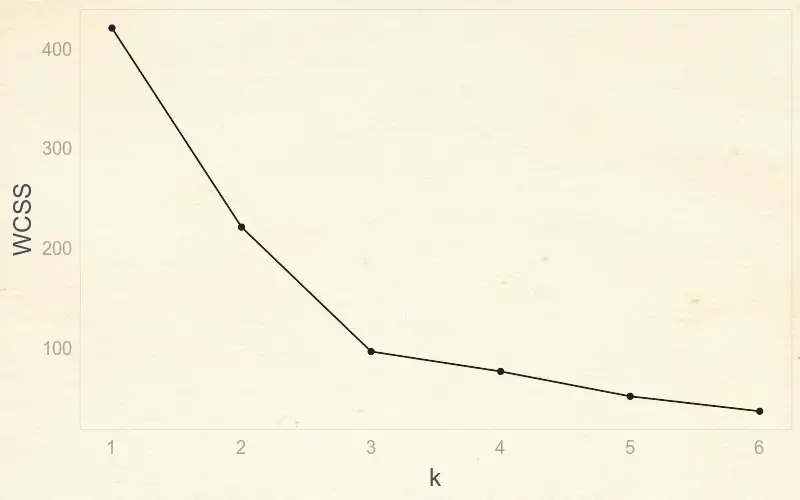
Using this graph, we can find the optimal value of k simply by locating the “elbow” of the curve. In the example, the optimal value will be 3. In fact, up to 3 there is a huge decrease in variation, while after this value the variation decreases much more slowly.
Where to use K-Means?
The k-Means does not require dedicated hardware and long data processing times. Therefore, the application fields are varied. For example, it is used to group GPS data to identify “hot” areas where different recordings occur. Another interesting application is image processing. Think of having to pixelate an image. Using K-means, with some care, and by appropriately defining the number of clusters (grid) you want to generate you can the following images.
Original image

Pixellated image by k-means

