
In many application contexts, we need to analyze data to extract useful information. For example, we might create classification models of insurance customers to assign the correct risk class to new customers. In other cases, we may be interested in clustering GPS data from vehicles to identify highly frequented and/or high-traffic areas. There are a plethora of algorithms for analyzing from the from algorithms ranging from classifiers to neural networks, from association rules to clustering. In this paper we will address a clustering algorithm called DBSCAN (Density-based spatial clustering of applications with noise).
As the name suggests, DBSCAN identifies clusters based on the density of points. Clusters are usually found in high-density regions, while outliers tend to be found in low-density regions. The three main advantages of its use (according to the originators of this algorithm) are:
- it requires minimal knowledge of the domain
- it can discover clusters of arbitrary shape
- is efficient for large databases
Below we will find out how it works step by step.
Algorithm
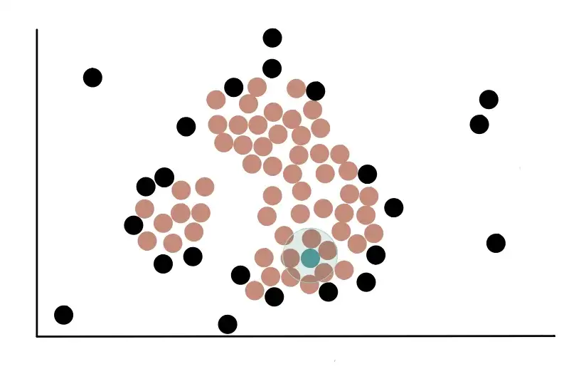
Suppose our raw data look like this:

The first thing to do is to count the number of points close to each point. Proximity is determined by drawing a circle of a certain radius (eps) around a point, and every other point that falls in this circle is said to be close to the first point. For example, we start with this red point and draw a circle around it.

We see that the circle drawn for this point includes, completely or partially, to other 7 points. So we can say that the red point is close to 7 points.
The radius of the circle, called eps, is the first parameter of the DSBCAN algorithm that we need to define. The choice of the value of eps is crucial. In fact, if we choose a value that is too small, much of the data will not be clustered. On the other hand, if we choose a value that is too large, the clusters will merge and many of our data points will be in the same cluster. In general, a smaller eps value is preferable.
Let us now consider this green dot. We see that it is close to 3 points because its circle with radius eps overlaps with 3 other points.

In the same way we proceed for all the remaining points, counting the number of neighboring points. Once this is done, we need to decide which points are core points and which are not.
This is where the second parameter of the algorithm comes into play: minPoints. We use minPoints to determine whether a point is a core point or not. If we set minPoints to 4, we say that a point is a core point if at least 4 points are neighbors to it. If the number of neighbors of a point is less than 4, it is considered a non-core point.
As a rule of thumb, minPoints ≥ number of dimensions in a dataset + 1. Larger values are generally better for datasets with noise. The minimum value of minPoints should be 3, but the larger our dataset, the larger the value of minPoints should be.
For our example, we set the value of minPoints to 4. In this way we can say that the red point is a Core Point because at least 4 points are close to it, while the green point is a Non-Core Point because only 3 points are close to it.
Ultimately, using the above process, we can determine that the following highlighted points are Core points.

Black dots, on the other hand, are Non-Core Points.
Now we randomly select a core point and assign it to the first cluster. Here, we randomly select a point and assign it to the green cluster.

Core points that are close to the green cluster, that is, that overlap the circle with radius eps will be added to the green cluster.
Therefore, core points close to the green cluster that is gradually growing are added to it. In the example below, we can see that 2 core points and 1 Non-Core Point are close to the green cluster. Only the 2 core points will be added to the cluster.

Eventually, all core points that are close to the green cluster will be added to it, and the data will appear like this:

Finally, all Non-Core Points close to the green cluster are added. For example, these 2 Non-Core Points are close to the blue cluster, so they are added:

However, since they are not core points, we do not use them to further extend the blue cluster. This means that the other Non-Core Point near Non-Core Point 1 will not be added to the green cluster.

Thus, unlike core points, Non-Core Points can only join a cluster but cannot be used to extend it further.
After adding all the Non-Core Points, we created our blue cluster, which looks like this:

Since none of the remaining core points are near the first cluster, we begin the process of forming a new cluster. First, we randomly choose a core point (which is not in a cluster) and assign it to our second yellow cluster.

We then add all the core points near the yellow cluster and use them to extend the cluster further.

Finally, the Non-Core Points located near the yellow cluster are added. After doing this, our data with the 2 clusters appear like this:

We keep repeating this process of creating clusters until there are no more core points. In our case, since all core points have been assigned to a cluster, we have finished creating new clusters. The remaining Non-Core Points that are not close to the core points and are not part of any cluster are called outliers.
In this way, we created our 2 clusters and found the outliers as well.
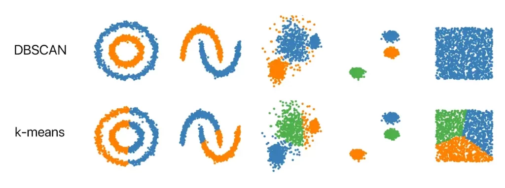
DBSCAN vs. K-Means vs. hierarchical clustering
There are also other types of clustering algorithms. The most popular ones are K-means and hierarchical clustering, which we will analyze in other articles. These two algorithms are used to identify compact, well-separated, globular-shaped clusters. They suffer, however, from the presence of noise and outliers in the data. On the other hand, DBSCAN captures complex-shaped clusters and does a very good job of identifying outliers. Another positive aspect of DBSCAN is that, unlike K-Means, it is not necessary to specify the number of clusters (k): the algorithm finds them automatically. The figure below shows some examples of datasets and the different results obtained using DBSCAN and k-means. It can be inferred that in some contexts (globular and well-separated clusters) the two algorithms obtain similar results, while in other cases it is appropriate to choose the algorithm that shows more robust behavior with respect to data distribution.


2 Responses