Analyzing data is one of the main tasks of data scientists. There are several libraries and tools that can be used depending on our needs. In the Python language, one of the most widely used libraries is Pandas. Pandas is an open-source library that provides a rich collection of data analysis tools. Much of its functionality is derived from the NumPy library. But why is it used instead of Numpy? Its features make it possible to:
- efficiently explore data
- handle missing data appropriately
- support different file formats such as CSV, JSON, Excel, etc.
- efficiently merge different data sets for smooth analysis
- read and write data during analysis
In this article we will focus on how to set up our work environment, the types of data structures available, and how to load different data formats. Let’s get started!
Configuration of the work environment
The fastest way to use Pandas is to download and install the Anaconda distribution. The Anaconda distribution of Python contains Pandas and various data analysis packages.
If you have Python and pip installed, run the following command from the terminal.
pip install pandas
You can of course also use Pandas in other work environments suitable for your project. You can use, for example, Jupyter notebook if you want to test your code by also including a workflow and comments. Or, if you need more computing power for your analysis we recommend using Google Colab.
To start using Pandas, you need to import it:
import pandas as pd
In this case we use pd as an alias for the Pandas library, which is usually quite used by programmers. Once the library is imported we can start working with it. Let us now explore the available data structures.
Data structures
Pandas has two main data structures, Series and DataFrame. These two data structures are built on NumPy arrays, which makes them fast for data analysis.
A Series is a labeled one-dimensional array structure that, in most cases, can be displayed as a column in an Excel spreadsheet.
A DataFrame is a two-dimensional array structure and is mostly represented as a table.
Create and retrieve data from a Series
We can convert basic Python data structures such as lists, tuples, dictionaries, and NumPy arrays into a Pandas series. The series has row labels representing the index.
We construct a Pandas series using the constructor pandas.Series( data, index, dtype, copy) where:
- data is a list, ndarray, tuple, etc.
- index is a unique, hashable value
- dtype is the data type
- copy is a copy of the data
					import numpy as np
import pandas as pd

sample_list_to_series = pd.Series([300, 240, 160]) # pass in the python list into Series method
print(sample_list_to_series)

'''
0    300
1    240
2    160
dtype: int64
'''

sample_ndarray_to_series = pd.Series(np.array([90, 140, 80])) # pass the numpy array in the Series method
print(sample_ndarray_to_series)

'''
0     90
1    140
2     80
dtype: int64
'''
The values in the series have been labeled with their index numbers, that is, the first value with index 0, the second with index 1, and so on. We can use these index numbers to retrieve a value from the series.
					print(sample_list_to_series[1])
# 240

print(sample_ndarray_to_series[2])
# 80
When working with series data, it is not necessary to work only with the default index assigned to each value. We can label each of these values as we wish, using the index argument.
					import numpy as np
import pandas as pd

sample_list_to_series = pd.Series([300, 240, 160], index = ['Ninja_HP', 'BMW_HP', 'Damon_HP'])
print(sample_list_to_series)
'''
Ninja_HP    300
BMW_HP      240
Damon_HP    160
dtype: int64
'''

sample_ndarray_to_series = pd.Series(np.array([90, 140, 80]), index = ['valx', 'valy', 'valz'])
print(sample_ndarray_to_series)
'''
valx     90
valy    140
valz     80
dtype: int64
'''
Then you can retrieve the data with the index label values in this way:
					print(sample_list_to_series['BMW_HP'])
# 240

print(sample_ndarray_to_series['valy'])
# 140
Note that with dictionaries it is not necessary to specify the index. Since a Python dictionary consists of key-value pairs, the keys will be used to create the index of values.
					sample_dict = {'Ninja_HP': 300, 'BMW_HP': 240, 'Damon_HP': 160}
print(pd.Series(sample_dict))
'''
Ninja_HP    300
BMW_HP      240
Damon_HP    160
dtype: int64
'''
To retrieve more data, a list of index label values like this is used:
					print(sample_list_to_series[['Ninja_HP', 'Damon_HP']])
'''
Ninja_HP    300
Damon_HP    160
dtype: int64
'''
Create and retrieve data from a DataFrame
Data in a DataFrame are organized in the form of rows and columns. You can create a DataFrame from lists, tuples, NumPy arrays, or from an array. However, in most cases, the DataFrame is created from dictionaries using the constructor pandas.DataFrame( data, index, columns, dtype, copy), where columns specifies column labels.
Creating a DataFrame from a list dictionary
If our dictionary contains lists, they must be the same length, otherwise an error will be thrown.
					dict_of_lists = {'model' : ['Bentley', 'Toyota', 'Audi', 'Ford'], 'weight' : [1400.8, 2500, 1600, 1700]}
data_frame = pd.DataFrame(dict_of_lists)
print(data_frame)
'''
     model  weight
0  Bentley  1400.8
1   Toyota  2500.0
2     Audi  1600.0
3     Ford  1700.0
'''
If no index specification is passed in the DataFrame method, the default index is passed with range(n), where n is the length of the list. In most cases, this is not what we want, so we will create an indexed DataFrame.
					dict_of_lists = {'Model' : ['Bentley', 'Toyota', 'Audi', 'Ford'], 'Weight' : [1400.8, 2500, 1600, 1700]}
indexed_data_frame = pd.DataFrame(dict_of_lists, index = ['model_1', 'model_2', 'model_3', 'model_4'])
print(indexed_data_frame)
'''
           Model  Weight
model_1  Bentley  1400.8
model_2   Toyota  2500.0
model_3     Audi  1600.0
model_4     Ford  1700.0
'''
Create a DataFrame from a dictionary of Series
We can create a DataFrame from a series.
					dict_of_series = {'HP': pd.Series([300, 240, 160], index = ['Ninja', 'BMW', 'Damon']), 'speed' : pd.Series(np.array([280, 300, 260, 200]), index = ['Ninja', 'BMW', 'Damon', 'Suzuki'])}
print(pd.DataFrame(dict_of_series))
'''
           HP  speed
BMW     240.0    300
Damon   160.0    260
Ninja   300.0    280
Suzuki    NaN    200
'''
As you can see, in the HP series, there is no value for the ‘Suzuki index since the series contains only 3 values. As a result, NaN will be added in the results without raising any error.
Selecting, adding and deleting columns
Accessing a column is as simple as accessing a value from a Python dictionary. You pass its name to the DataFrame, which returns the results in the form of pandas.Series.
					dict_of_lists = {'Model' : ['Bentley', 'Toyota', 'Audi', 'Ford'], 'Weight' : [1400.8, 2500, 1600, 1700]}
indexed_data_frame = pd.DataFrame(dict_of_lists, index = ['model_1', 'model_2', 'model_3', 'model_4'])
print(indexed_data_frame['Weight']) # get the weights column
'''
model_1    1400.8
model_2    2500.0
model_3    1600.0
model_4    1700.0
Name: Weight, dtype: float64
'''
It is possible, however, to add a column to an existing DataFrame using a new Pandas series. In the following example, we add the fuel consumption for each motorcycle in the DataFrame.
					dict_of_series = {'HP': pd.Series([300, 240, 160], index = ['Ninja', 'BMW', 'Damon']), 'speed' : pd.Series(np.array([280, 300, 260, 200]), index = ['Ninja', 'BMW', 'Damon', 'Suzuki'])}
bikes_data_df= pd.DataFrame(dict_of_series)
#add column of fuel consumption
bikes_data_df['Fuel Consumption'] = pd.Series(np.array(['27Km/L', '24Km/L', '30Km/L', '22Km/L']), index = ['Ninja', 'BMW', 'Damon', 'Suzuki']) #add column of fuel consumption
print(bikes_data_df)
'''
           HP  speed Fuel Consumption
BMW     240.0    300           24Km/L
Damon   160.0    260           30Km/L
Ninja   300.0    280           27Km/L
Suzuki    NaN    200           22Km/L
'''
Columns can also be deleted from the DataFrame. To do this, the pop or del functions can be used. We remove the speed and fuel consumption columns from the Motorcycle DataFrame.
					# using pop function
bikes_data_df.pop('speed')
print(bikes_data_df)
'''
           HP Fuel Consumption
BMW     240.0           24Km/L
Damon   160.0           30Km/L
Ninja   300.0           27Km/L
Suzuki    NaN           22Km/L
'''

#using delete function
del bikes_data_df['Fuel Consumption']
print(bikes_data_df)
'''
           HP
BMW     240.0
Damon   160.0
Ninja   300.0
Suzuki    NaN
'''
Selecting, adding and deleting rows
Pandas has the loc and iloc operators, which can be used to access rows in a DataFrame.
iloc makes a selection based on the index. It selects a row based on its position within the DataFrame. In the following code, for example, data from the second row of the DataFrame is selected.
					dict_of_series = {'HP': pd.Series([300, 240, 160], index = ['Ninja', 'BMW', 'Damon']), 'speed' : pd.Series(np.array([280, 300, 260, 200]), index = ['Ninja', 'BMW', 'Damon', 'Suzuki'])}
bikes_data_df= pd.DataFrame(dict_of_series)
bikes_data_df.iloc[1]
'''
HP       160.0
speed    260.0
Name: Damon, dtype: float64
'''
loc makes a selection based on labels instead. It selects a row based on the data index value and not based on location. In the following example, we select data from the row with the label BMW.
					dict_of_series = {'HP': pd.Series([300, 240, 160], index = ['Ninja', 'BMW', 'Damon']), 'speed' : pd.Series(np.array([280, 300, 260, 200]), index = ['Ninja', 'BMW', 'Damon', 'Suzuki'])}
bikes_data_df= pd.DataFrame(dict_of_series)
bikes_data_df.loc['BMW']
'''
HP       240.0
speed    300.0
Name: BMW, dtype: float64
'''
The append function to the DataFrame is used to add a new row.
Attention!
New rows will always be added to the end of the original DataFrame.
					sample_dataframe1 = pd.DataFrame([['Ninja',280],['BMW',300],['Damon',200]], columns = ['Model','Speed'])
sample_dataframe2 = pd.DataFrame([['Suzuki', 260], ['Yamaha', 180]], columns = ['Model','Speed'])
sample_dataframe1 = sample_dataframe1.append(sample_dataframe2)
print(sample_dataframe1)
'''
    Model  Speed
0   Ninja    280
1     BMW    300
2   Damon    200
0  Suzuki    260
1  Yamaha    180
'''
Reading and analyzing data
In the previous section we looked at the two main data structures in Pandas: Series and DataFrame. In the previous examples we entered the data directly from code because we wanted to focus on the data structures and how to read and manipulate them. Hardly in real cases will we write data directly from code, but we will have to read it from external sources.
There are many formats in which data can be stored, but in this article we will look at the following types of data formats:
- CSV (Comma Separated Values) files.
- JSON files.
- SQL database files.
- Excel files.
Reading and analyzing data from a CSV file
We use the Melbourne housing market dataset from Kaggle. We will download the data to our notebook in Colab using the API provided by Kaggle.
To do this you must first log into your Kaggle account (create one if you do not have one) and from your profile settings create an API Key.

Now load the kaggle.json file that was automatically loaded into the root folder of the Colab notebook. Once loaded perform the following instructions.
					! mkdir ~/.kaggle
! cp kaggle.json ~/.kaggle/
! chmod 600 ~/.kaggle/kaggle.json
! kaggle datasets download anthonypino/melbourne-housing-market
! unzip melbourne-housing-market.zip
At this point we have the data available in our workspace and can load it. To load the data from the CSV file, we use pd.read_csv().
					melbourne_data = pd.read_csv('/content/Melbourne_housing_FULL.csv')
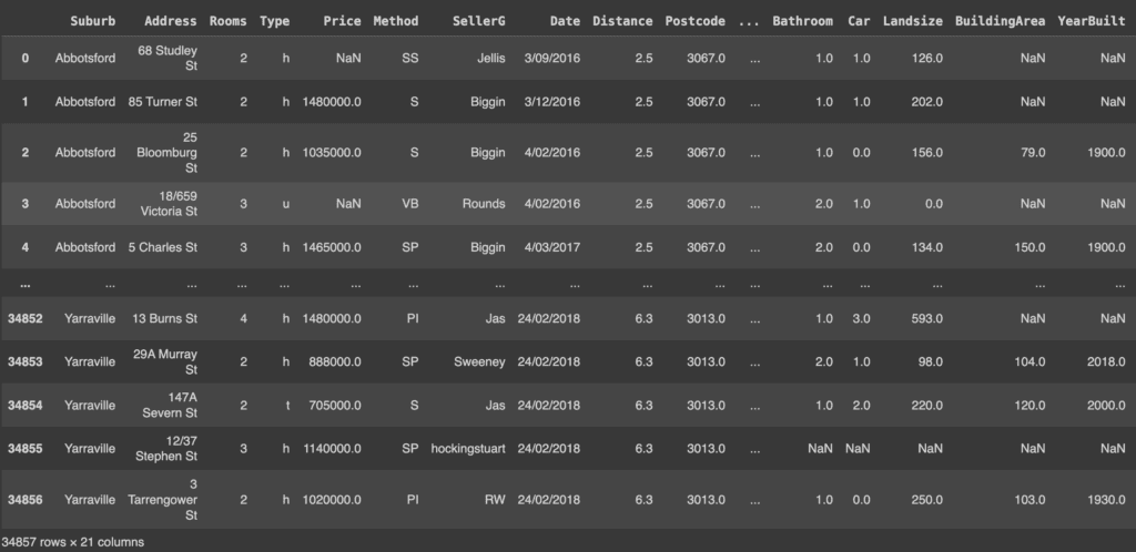
melbourne_data

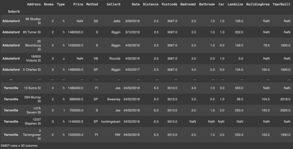
The results show that Pandas created its own index column (the first column displayed) even though the CSV file has its own index column (the Suburb attribute). In order for Pandas to use the CSV index column, index_col must be specified.
					melbourne_data = pd.read_csv('/content/Melbourne_housing_FULL.csv', index_col=0)
melbourne_data

If you want to reset the index to the normal index (0, 1… etc.), you can use the reset_index() method. This method resets the index of the DataFrame to zero and uses the default index.
melbourne_data.reset_index()
Note that the Suburb index is returned as a column. However, in the following examples we will proceed with an indexed DataFrame.
Since the data is huge and represented in a DataFrame, Pandas returns only the first five rows and the last five rows. We can check the size of the data using the shape attribute.
					print(melbourne_data.shape)
# (34857, 21)
The DataFrame has 34857 records (rows) and 21 columns. You can examine any number of records using the head() method. By default, this method displays the first five records.
melbourne_data.head()

If, on the other hand, we want to display only a predefined number of initial rows (e.g. 3) we will use the following command.
melbourne_data.head(3)

Similarly if we want to display the last few rows of our DataFrame we can use the tail() method. By default, it returns the last five records, but we can pass the number of rows we want to display.
melbourne_data.tail(3)

To get more information about the dataset, you can use the info() method. This method prints the number of entries in the dataset and the data type of each column.
					print(melbourne_data.info())
'''
<class "pandas.core.frame.DataFrame">
Index: 34857 entries, Abbotsford to Yarraville
Data columns (total 20 columns):
 #   Column         Non-Null Count  Dtype
---  ------         --------------  -----
 0   Address        34857 non-null  object
 1   Rooms          34857 non-null  int64
 ...
 18  Regionname     34854 non-null  object
 19  Propertycount  34854 non-null  float64
dtypes: float64(12), int64(1), object(7)
memory usage: 5.6+ MB
None
'''
Reading data from a JSON file
In Pandas it is also possible to read data in json format. For this purpose we create a simple JSON file with Python and read it with Pandas.
					import json

# creating a simple JSON file
car_data ={
        'Porsche': {
        'model': '911',
        'price': 135000,
        'wiki': 'http://en.wikipedia.org/wiki/Porsche_997',
        'img': '2004_Porsche_911_Carrera_type_997.jpg'
    },'Nissan':{
        'model': 'GT-R',
        'price': 80000,
        'wiki':'http://en.wikipedia.org/wiki/Nissan_Gt-r',
        'img': '250px-Nissan_GT-R.jpg'
    },'BMW':{
        'model': 'M3',
        'price': 60500,
        'wiki':'http://en.wikipedia.org/wiki/Bmw_m3',
        'img': '250px-BMW_M3_E92.jpg'
    },'Audi':{
        'model': 'S5',
        'price': 53000,
        'wiki':'http://en.wikipedia.org/wiki/Audi_S5',
        'img': '250px-Audi_S5.jpg'
    },'Audi':{
        'model': 'TT',
        'price': 40000,
        'wiki':'http://en.wikipedia.org/wiki/Audi_TT',
        'img': '250px-2007_Audi_TT_Coupe.jpg'
    }
}
jsonString = json.dumps(car_data)
jsonFile = open("cars.json", "w")
jsonFile.write(jsonString)
jsonFile.close()
Now in our folder we have a cars.json file.
To read the data from the JSON file, we use pd.read_json(). Pandas will automatically convert the dictionary object to a DataFrame and define the column names separately.
pd.read_json('/content/cars.json')

The head() and tail() methods can be applied to analyze the data, as we did for CSV files.
Reading data from a SQL database
In many contexts, data are available in relational databases. For this example, we create a database with python sqlite3. Pandas uses the read_sql_query() method to convert the data to a DataFrame.
First, we connect to SQLite, create a table, and enter values.
					import sqlite3
conn = sqlite3.connect('vehicle_database')
c = conn.cursor()
# let's create a table and insert values with sqlite3
c.execute('''
          CREATE TABLE IF NOT EXISTS vehicle_data
          ([vehicle_id] INTEGER PRIMARY KEY, [vehicle_model] TEXT, [weight] INTEGER, [color] TEXT)
          ''')
conn.commit()
# insert values into tables
c.execute('''
          INSERT INTO vehicle_data (vehicle_id, vehicle_model, weight, color)
                VALUES
                (1,'Bentley',1400,'Blue'),
                (2,'Toyota',2500,'Green'),
                (3,'Audi',1600,'Black'),
                (4,'Ford',1700,'White')
          ''')
conn.commit()
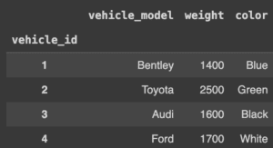
In the vehicle database, we have a table called vehicle_data. We will pass the SELECT statement and the conn variable to read from that table.
					cars_df = pd.read_sql_query("SELECT * FROM vehicle_data", conn)
cars_df.set_index('vehicle_id') # set index to vehicle_id

Reading data from an Excel file
It is also possible to read data from excel sheets. To create an excel file directly from Python we must first install the XlsxWriter module via the following command.
! pip install xlsxwriter
At this point we can create our example excel file.
					import xlsxwriter
workbook = pd.ExcelWriter('students.xlsx', engine='xlsxwriter')
workbook.save()

try:
  df = pd.DataFrame({'stud_id': [1004, 1007, 1008, 1100],
      'Name': ['Brian', 'Derrick', 'Ann', 'Doe'],
      'Age': [24, 26, 22, 25]})
  workbook = pd.ExcelWriter('students.xlsx', engine='xlsxwriter')
  df.to_excel(workbook, sheet_name='Sheet1', index=False)
  workbook.save()
except:
  print('Excel sheet exists!')
We have thus created an Excel file called students.xlsx. To read data from an Excel file we use the read_excel() method.
					stud_data = pd.read_excel('/content/students.xlsx')
stud_data.set_index('stud_id')


One Response