In the previous article Pandas: data analysis with Python [part 1]., we introduced Pandas and its data structures. We then focused on how to read data and manipulate it from different data sources. Of course, the Python library is designed to analyze data. In this paper we will look at some aspects of data analysis that the library provides us with. In particular, we will discuss how to clean the data, extract statistics, create pivot tables, and graph the results.
The examples we will look at will use the data we have already downloaded and loaded in article Pandas: data analysis with Python [part 1].. You can go read it if you need to reset your work environment and/or load the necessary data from Kaggle. Once you have uploaded the data you can get started!
Data cleaning
In data science, we used to extract information from huge volumes of raw data. This raw data may contain “dirty” and inconsistent values, leading to inaccurate analysis and unhelpful insights. In most cases, the initial stages of data acquisition and cleaning can make up 80 percent of the work; therefore, if you intend to enter this field, you must learn how to handle “dirty” data.
Data cleaning focuses primarily on removing erroneous, corrupt, improperly formatted, duplicate, or incomplete data within a dataset.
In this section, we will address the following:
- removal of unnecessary columns from the dataset
- removal of duplicates
- finding and replacing missing values in the DataFrame
- modifying the index of the DataFrame
- renaming columns in a DataFrame.
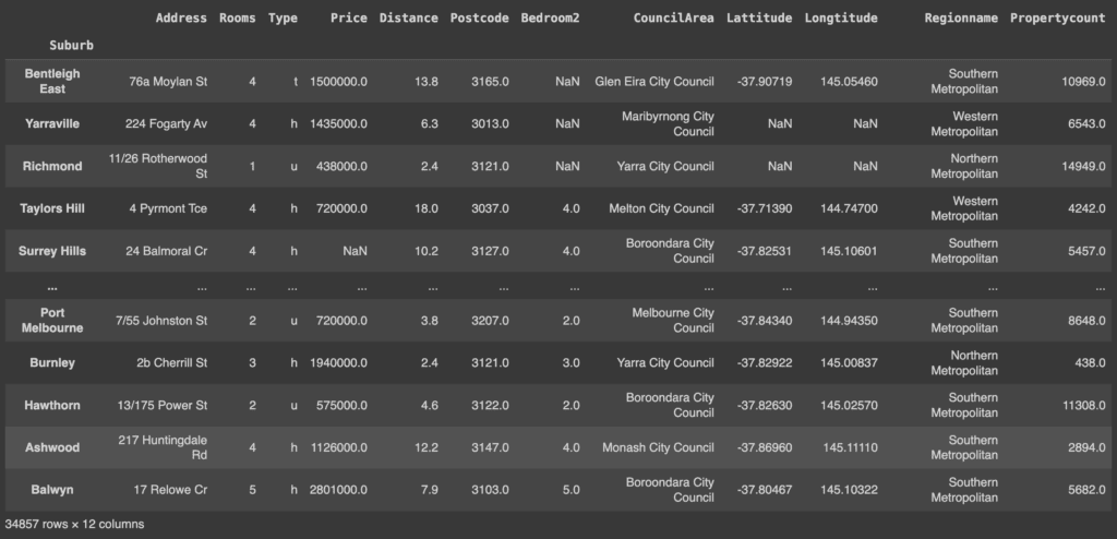
We use the Melbourne housing market dataset imported from Kaggle. First, we shuffle the DataFrame to get rows with different indexes. To reproduce the same shuffled data each time, we use a random_state.
					shuffled_melbourne_data = melbourne_data.sample(frac=1, random_state=1) # produce the same shuffled data each time
shuffled_melbourne_data

Suppose that in the DataFrame you want to get information about:
- What are the best suburbs in which to buy?
- The suburbs with good value for money?
- What is the expensive side of town?
- Where to buy a two-bedroom unit?
We may need all but the following columns:
- Method
- SellerG
- Date
- Bathroom
- Car
- Landsize
- BuildingArea
- YearBuilt
Pandas has a drop() method to remove these columns.
					# Define a list names of all the columns we want to drop
columns_to_drop = ['Method',
                   'SellerG',
                   'Date',
                   'Bathroom',
                   'Car',
                   'Landsize',
                   'BuildingArea',
                   'YearBuilt']
shuffled_melbourne_data.drop(columns = columns_to_drop, inplace=True, axis=1)
shuffled_melbourne_data
Attention!
The option (inplace = True) ensures that the method does not return a new DataFrame, but looks for columns to remove from the given DataFrame. True means that the change is permanent.
Colonne eliminate!
Finding and removing duplicates
The duplicated() method returns boolean values in column format. False values mean that no data has been duplicated.
					shuffled_melbourne_data.duplicated()
'''
Suburb
Bentleigh East    False
                  ...
Balwyn            False
Length: 34857, dtype: bool
'''
This duplicate check can be performed for small DataFrames. For larger DataFrames, it is impossible to check every single value. Therefore, we will concatenate the any() method to duplicated().
					shuffle_melbourne_data.duplicated().any()
# True
If the any() method returns True, it means that there are duplicates in the DataFrame. To remove them, we will use the drop_duplicates() method.
					shuffled_melbourne_data.drop_duplicates(inplace=True) # remove dupicates
shuffled_melbourne_data.duplicated().any() # Checking returns False
# False
Find and replace missing values in the DataFrame
Four methods are available to check for missing values, i.e., taking the value null. They are:
- isnull(): returns a data set with boolean values.
shuffled_melbourne_data.isna()

- isna(): similar to isnull()
- isna().any(): returns a column format of boolean values
					shuffled_melbourne_data.isna().any()
'''
Address          False
Rooms            False
Type             False
Price             True
Distance          True
Postcode          True
Bedroom2          True
CouncilArea       True
Lattitude         True
Longtitude        True
Regionname        True
Propertycount     True
dtype: bool
'''
- isna().sum(): returns a column total of all available nulls.
					shuffled_melbourne_data.isna().sum()
'''
Address             0
Rooms               0
Type                0
Price            7580
Distance            1
Postcode            1
Bedroom2         8202
CouncilArea         3
Lattitude        7961
Longtitude       7961
Regionname          3
Propertycount       3
dtype: int64
'''
Missing values can be handled in two ways:
- By removing the rows that contain the missing values.
In this case we use the dropna() method to remove the rows. For the following examples we will not yet remove rows in our dataset.
shuffled_melbourne_data.dropna(inplace=True) # removes all rows with null values
- Replacing empty cells with new values
We can decide to replace all null values with a value using the fillna() method. The syntax is DataFrame.fillna(value, method, axis, inplace, limit, downcast) where the value can be a dictionary that takes the column names as the key.
					shuffled_melbourne_data.fillna({'Price':1435000, 'Distance':13, 'Postcode':3067, 'Bedroom2': 2, 'CouncilArea': 'Yarra City Council'}, inplace=True)
print(shuffled_melbourne_data.isna().sum())
'''
Address             0
Rooms               0
Type                0
Price               0
Distance            0
Postcode            0
Bedroom2            0
CouncilArea         0
Lattitude        7961
Longtitude       7961
Regionname          3
Propertycount       3
dtype: int64
'''
We have successfully replaced the specified empty values of the dictionary columns within the fillna() method.
Changing the index of the DataFrame
When working with data, you usually want a field with a unique value as an index to the data. For example, in our cars.json dataset, you can assume that when a person searches for a record of a car, they will probably search for it by its model (values in the Model column).
La verifica se la colonna del modello ha valori univoci restituisce True, quindi sostituiamo l’indice esistente con questa colonna usando set_index:
					cars = pd.read_json('/content/cars.json', orient=’index’)

print(cars['model'].is_unique)
# True
cars.set_index('model', inplace=True)

Now each record can be accessed directly with loc[].
					cars.loc['M3']
'''
price                                  60500
wiki     http://en.wikipedia.org/wiki/Bmw_m3
img                     250px-BMW_M3_E92.jpg
Name: M3, dtype: object
'''
Renaming columns in a DataFrame
Sometimes you may want to rename data columns for better interpretation, perhaps because some names are not easy to understand. To do this, you can use the rename() method of the DataFrame and pass a dictionary where the key is the current column name and the value is the new name.
Let’s use the original Melbourne DataFrame, in which no column has been removed. We may want to rename:
- Room to No_ofRooms.
- Type to HousingType.
- Method to SaleMethod
- SellerG to RealEstateAgent.
- Bedroom2 to No_ofBedrooms.
					# Use initial Melbourne DataFrame
#Create a dictionary of columns to rename. Value is the new name
columns_to_rname = {
    'Rooms': 'No_ofRooms',
    'Type': 'HousingType',
    'Method': 'SaleMethod',
    'SellerG': 'RealEstateAgent',
    'Bedroom2': 'No_ofBedrooms'
}
shuffled_melbourne_data.rename(columns=columns_to_rename, inplace=True)
shuffled_melbourne_data.head()

Finding correlations
Pandas has a corr() method that allows us to find relationships between columns in our data set.
The method returns a table representing the relationship between two columns. The values range from -1 to 1, where -1 indicates a negative correlation and 1 a perfect correlation. The method automatically ignores null values and nonnumeric values in the data set.
shuffled_melbourne_data.corr()

Descriptive statistics
There are several methods in Pandas DataFrames and Series to perform summary statistics. These methods include: mean, median, max, std, sum and min.
For example, we can find the mean of the price in our DataFrame.
					shuffled_melbourne_data['Price'].mean()
# 1134144.8576355954
# Or for all columns
shuffled_melbourne_data.mean()
No_ofRooms       3.031071e+00
Price            1.134145e+06
				 ...
Propertycount    7.570273e+03
dtype: float64
If we want to get an overview of basic statistics, which include those mentioned above, for all the attributes of our data we can use the describe() method.
shuffled_melbourne_data.describe()

Groupby operation to split, aggregate and transform data
The Pandas groupby() function allows you to reorganize data. It simply divides the data into groups classified according to some criteria and returns a set of DataFrame objects.
Divide data into groups
Let us divide the Melbourne data into groups based on the number of bedrooms. To display the groups, we use the groups attribute.
					grouped_melb_data = shuffled_melbourne_data.groupby('No_ofBedrooms')
shuffled_grouped_melb_data.groups
'''
{1.0: ['Hawthorn', 'St Kilda'], 2.0: ['Bentleigh East', 'Yarraville', 'Richmond', 'Mill Park', 'Southbank', 'Surrey Hills', 'Caulfield North', 'Reservoir', 'Mulgrave', 'Altona', 'Ormond', 'Bonbeach', 'St Kilda', 'South Yarra', 'Malvern', 'Essendon'],
...
30.0: ['Burwood']}}
'''
Since the result is a dict and the data is huge, the result is difficult to read. To overcome this problem, we can use the keys() method to get only the keys representing the groups.
					grouped_melb_data.groups.keys()
# dict_keys([0.0, 1.0, 2.0, 3.0, 4.0, 5.0, 6.0, 7.0, 8.0, 9.0, 10.0, 12.0, 16.0, 20.0, 30.0])
We can also group multiple columns as follows.
					grouped_melb_data = shuffled_melbourne_data.head(20).groupby(['No_ofBedrooms', 'Price'])
grouped_melb_data.groups.keys()
'''
dict_keys([(1.0, 365000.0), (1.0, 385000.0), (2.0, 380000.0), (2.0, 438000.0), ... (4.0, 1435000.0)])
If we want to select a group of our interest, we will use the get_group() method.
					grouped_melb_data = melbourne_data.groupby('No_ofBedrooms')
grouped_melb_data.get_group(2) # select 2 bedrooms group

Aggregated data
An aggregate function returns a single collective value for each group. For example, we wish to calculate the average price for each group. We will use the agg function.
					print(grouped_melb_data['Price'].agg([np.mean]))
'''
                       mean
No_ofBedrooms
0.0            1.054029e+06
1.0            6.367457e+05
			   ...
30.0           1.435000e+06
'''
Transformation
Pandas has a transformation operation that is used with the groupby() function. This allows the data to be summarized effectively. When we transform a group, we get an indexed object of the same size as the one being grouped. For example, in our data set, we can get the average prices for each No_ofBedrooms group and combine the results in our original data set for other calculations.
The first approach would be to try to group the data in a new DataFrame and combine them in a multi-step process, and then combine the results in the original DataFrame. We would create a new DataFrame with average prices and merge it back with the original.
					price_means = shuffled_melbourne_data.groupby('No_ofBedrooms')['Price'].mean().rename('MeanPrice').reset_index()
df_1 = shuffled_melbourne_data.merge(price_means)
df_1

Complex? We can then use the transform operator to perform the same operation in one step.
					shuffled_melbourne_data['MeanPrice'] = shuffled_melbourne_data.groupby('No_ofBedrooms')['Price'].transform('mean')
shuffled_melbourne_data

Pivot table
A Pandas pivot table is similar to the groupby operation. It is a common operation for programs that use tabular data such as spreadsheets. The difference between the groupby operation and the pivot table is that a pivot table takes simple columnar data as input and groups the entries into a two-dimensional table that provides a multidimensional summary of the data. Its syntax is:
pandas.pivot_table(data, values=None, index=None, columns=None, aggfunc=’mean’, fill_value=None, margins=False, dropna=True, margins_name=’All’, observed=False)
Let us now create an example pivot table.
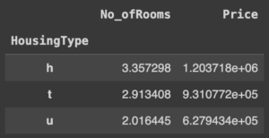
					pivot_tbl = shuffled_melbourne_data.pivot_table(index='HousingType')
pivot_tbl

What did we get? The result is a new DataFrame, called pivot_tbl, which is grouped by HousingType. Since no other parameters were specified in the function, the data was aggregated by the average for each column with numeric data, since by default the aggfunc parameter returns the average.
Aggregation of data by specific columns
It is also possible to aggregate data by specific columns. In the following example, we aggregate for Price and No_ofRooms columns.
					pivot_tbl = shuffled_melbourne_data.pivot_table(index='HousingType', values=['Price', 'No_ofRooms'])
pivot_tbl
Using aggregation methods in the pivot table
You can change the way the data are aggregated in the pivot table. Aggregation methods can thus be used to perform complex analyses. To use them, you must specify the aggregation function in the aggfunc parameter.
For example, if we want to find the sum of all property counts for each region ( Regionname attribute), we would use the following code.
					pivot_tbl_sum = shuffled_melbourne_data.pivot_table(index='Regionname', aggfunc='sum', values='Propertycount')
pivot_tbl_sum

Multiple aggregation methods
To apply multiple aggregation methods, a list of aggregation methods must be specified in the aggfunc parameter. For example , to find the sum and maximum number of properties for each region the code would be as follows.
					pivot_tbl_sum_max = shuffled_melbourne_data.pivot_table(index='Regionname', aggfunc=['sum', 'max'], values='Propertycount')
pivot_tbl_sum_max

Specify the aggregation method for each column
In the previous examples, we applied the same aggregation methods to one or more columns. To specify the aggregation function of interest for each column, we can use a dictionary containing the column as the key and the aggregation function as the value. Here is an example.
					pivot_tbl = shuffled_melbourne_data.pivot_table(index='Regionname', values=['Price', 'Propertycount'], aggfunc={'Price':'sum', 'Propertycount':'mean'})
pivot_tbl

Split data in pivot table by column with columns
A column can be added to the pivot table with the columns parameter. This divides the data horizontally, while the index parameter specifies the column to divide the data vertically. In the following example, the data are divided according to the type of dwelling.
					pivot_tbl = shuffled_melbourne_data.pivot_table(
				index='Regionname',
                values=['Price', 'Propertycount'],
                aggfunc={'Price':'sum', 'Propertycount':'mean'},
                columns='HousingType'
                )
pivot_tbl

Adding totals to each group
Sometimes it is necessary to add totals after aggregating. This is done by using the margins parameter. By default, it is set to False and its label is set to ‘All’. To rename it, we need to use the margin_name parameter. Let’s see how we can get the totals of all property counts for each region.
					pivot_tbl = shuffled_melbourne_data.pivot_table(
					index='Regionname',
                    values='Propertycount',
                    margins=True,
                    margins_name='Totals',
                    aggfunc='sum',
                    columns='HousingType')
pivot_tbl

As you may have noticed, the pivot table code is simpler and more readable than the groupby operation.
Sort DataFrames
Pandas provides a sort_values() method for sorting a DataFrame. The types of sorting that can be performed are as follows:
- ascending order
- descending order
- sorting by multiple columns
Increasing order
We sort the Melbourne data by price. By default, data are sorted in ascending order.
					shuffled_melbourne_data.sort_values(by=['Price'], inplace=True)
shuffled_melbourne_data.head(3)

Descending order
To sort in descending order, simply add the condition ascending=False to the sort_values() method. Let’s sort the Melbourne data by price.
					shuffled_melbourne_data.sort_values(by=['Price'], inplace=True, ascending=False)
shuffled_melbourne_data.head(3)

Sorting by multiple columns
To sort over multiple columns you must pass a list in the by parameter. The order of the list elements is important. In fact, if the value of the first element in the list is equal, we sort by the second attribute and so on. In the next example we sort by No_ofRooms and Price.
					shuffled_melbourne_data.sort_values(by=['No_ofRooms','Price'], inplace=True)
shuffled_melbourne_data.head(3)

Plot data
To create graphs, Pandas uses the plot() method. Since this method integrates with the Matplotlib library, we can use the Pyplot module for these visualizations.
First, we import the matplotlib.pyplot module and give it plt as an alias, then define some parameters of the figures that will be generated.
					import matplotlib.pyplot as plt
plt.rcParams.update({'font.size': 25, 'figure.figsize': (50, 8)}) # set font and plot size to be larger
There are different types of graphs for displaying information of interest. Below we see some examples that are most commonly used.
Scatter plot
The main purpose of a scatter plot is to check whether two variables are related. In this example we try to compare No_ofRooms and Price.
					shuffled_melbourne_data.plot(kind='scatter', x='No_ofRooms', y='Price', title='Price vs Number of Rooms')
plt.show()

A scatter plot is not a definitive proof of a correlation. To get an overview of the correlations between different columns, one can use the corr() method seen earlier.
Histograms
Histograms help visualize the distribution of values in a data set. They provide a visual interpretation of numerical data by showing the number of objects that fall within a specified range of values (called “bin”).
					shuffled_melbourne_data['Price'].plot(kind='hist', title='Pricing')
plt.show()

Pie charts
Pie charts show the percentages of data that fall into a particular group compared to the entire dataset.
					price_count = shuffled_melbourne_data.groupby('Address')['Price'].sum()
print(price_count) #price totals each group
'''
Address
1 Abercrombie St    1435000.0
1 Aberfeldie Wy      680000.0
                      ...
9b Stewart St       1160000.0
Name: Price, Length: 34009, dtype: float64
'''
small_groups = price_count[price_count < 1500000]
large_groups = price_count[price_count > 1500000]

small_sums = pd.Series([small_groups.sum()], index=["Other"])
large_groups = large_groups.append(small_sums)

large_groups.iloc[0:10].plot(kind="pie", label="")
plt.show()

Conversion to CSV, JSON, Excel or SQL
After working with the data, you may decide to convert the data from one format to another. Pandas has methods for making these conversions as easily as we read the data.
Convert JSON to CSV
To convert to CSV, we use the df.to_csv() method. So, to convert our cars.json file, we should proceed like this.
					cars = pd.read_json('cars.json', orient='index')
cars_csv = cars.to_csv(r'New path to where new CSV file will be stored\New File Name.csv', index=False) # disable index as we do not need it in csv format.
Convert CSV to JSON
We now convert to JSON using the pd.to_json() method.
					melbourne_data = pd.read_csv('Melbourne_housing_FULL.csv, orient-'index'
melbourne_data.to_json(r'New path to where new JSON file will be stored\New File Name.json')
Export a SQL table to CSV
We can also convert the SQL table to a CSV file:
					cars_df = pd.read_sql_query("SELECT * FROM vehicle_data", conn)
cars_df.to_csv(r'New path to where new csv file will be stored\New File Name.csv', index=False)
Convert CSV to Excel
CSV files can also be converted to Excel:
					melbourne_data = pd.read_csv('Melbourne_housing_FULL.csv, orient-'index')
melbourne_data.to_excel(r'New path to where new excel file will be stored\New File Name.xlsx', index=None, header=True)
Convert Excel to CSV
Similarly, Excel files can be converted to CSV:
					stud_data = pd.read_excel('/content/students.xlsx')
stud_data.to_csv(r'New path to where new csv file will be stored\New File Name.csv', index=None, header=True)
Convert DataFrame to SQL table
Pandas has the df.to_sql() method to convert a DataFrame to an SQL table.
					cars = pd.read_json('cars.json', orient='index')

from sqlalchemy import create_engine #pip install sqlalchemy
engine = create_engine('sqlite://', echo=False)

cars.to_sql(name='Cars', con=engine) # name='Cars' is the name of the SQL table